Bike sharing prediction using deep learning
The goal of this project is to predict the bike sharing count per hour
 Image credit: zamani.ai
Overview
bike-sharing
The goal is to predict the bike sharing count per hour. The dataset can be downloaded here
I have uploaded the source code in this repo: https://github.com/zamani/bike_sharing_prediction
Setup
⚠️update pip and install virtualenv if necessary (check here) (Optional) update the python pip
python -m pip install --upgrade pip
First clone the repo and navigate into the local repo:
git clone https://github.com/zamani/bike_sharing_prediction.git
cd bike_sharing_prediction
Create a virtual environment in python:
python -m venv bike_sharing_env
Then, activate the environment on Windows:
.\bike_sharing_env\Scripts\activate
(And on Linux/macOS)
source env/bin/activate
Finally, install the requirements:
pip install -r requirements.txt
Baselines
The proposed RNN method is compared with some simple baseline methods:
| Baseline Method | MAE | STD |
|---|---|---|
| Previous Hour Count | 85.06 | 97.70 |
| Previous Day, Same Hour | 81.08 | 108.48 |
| Keep Hourly Pace | 89.21 | 125.17 |
| Linear Regression, without regularization | 142.21 | 115.59 |
The results can be shown by running the following command
python baselines.py
Method
In this repository, I have used RNN-GRU with different configurations. The RNN architecture is chosen for this problem because considering the sequence of consequence features and the previous output gives us additional information (comparing with only current input features). This leads to a more accurate prediction and can be modeled by the RNN. First, the dataset is divided into 70% training set, 10% validation set and 20% test set. Then, the bike count is normalized respect to the maximum bike count number in the training set.
The network is trained with the relative count respect to the previous day (same hour) or the previous hour. It means in this approach we have one of these two assumptions: either (1) we already know the count of the previous hour and we need to predict the next hour or (2) we know the previous day data (which is more realistic). The proposed architecture calculates the relative change and its value is converted into the absolute value for getting the absolute count number. Also, the relative change was trained by converting them into discrete bins and use the representative of bins as the relative increase/decrease. Only the number of bins should be defined. The bins width are automatically selected in a way that each bin almost has the same number of samples. On the other hands bins can also be defined manually such as [-1]+[-.75:0.05:0.45]+[0.5:0.25:2.5].
Here are the results with Gated Recurrent Unit (GRU) on a fixed random seed:
| RNN-GRU input (output is Y(t)) | command (python main.py <ARGUMENTS>) |
MAE | STD |
|---|---|---|---|
| X(t) | -seqlen 1 |
82.42 | 132.94 |
| [X(t-1), X(t)] | -seqlen 2 |
75.53 | 140.15 |
| [X(t-2), X(t-1), X(t)] | -seqlen 3 |
92.69 | 162.90 |
| [X(t), Y(t-1)] | -seqlen 1 -prev_cnt hour |
43.78 | 71.26 |
| [[X(t-1), Y(t-2)], [X(t), Y(t-1)]] | -seqlen 2 -prev_cnt hour |
13.73 | 19.33 |
| [X(t), Y(t-24)] | -seqlen 1 -prev_cnt day -day_num 1 |
65.95 | 108.71 |
| [X(t), Y(t-24), Y(t-48)] | -seqlen 1 -prev_cnt day -day_num 2 |
33.15 | 33.15 |
| [[X(t-1), Y(t-25)], [X(t), Y(t-24)]] | -seqlen 2 -prev_cnt day -day_num 1 |
64.24 | 100.13 |
| [[X(t-1), Y(t-25), Y(t-49)], [X(t), Y(t-24), Y(t-48)]] | -seqlen 2 -prev_cnt day -day_num 2 |
18.98 | 34.17 |
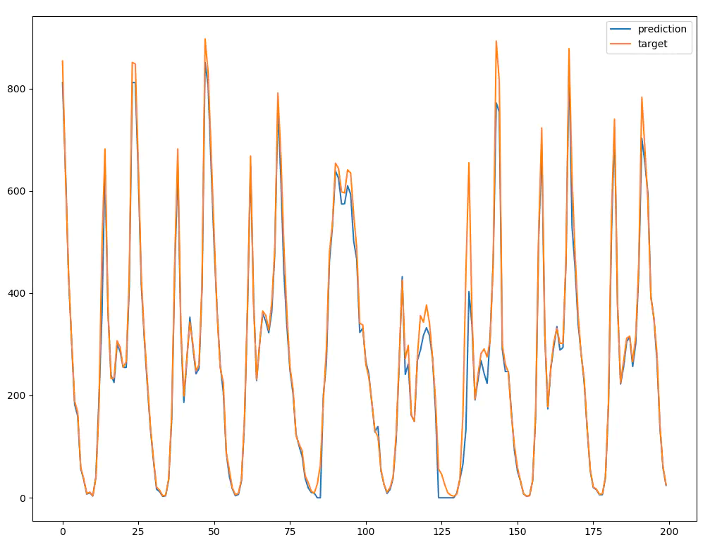
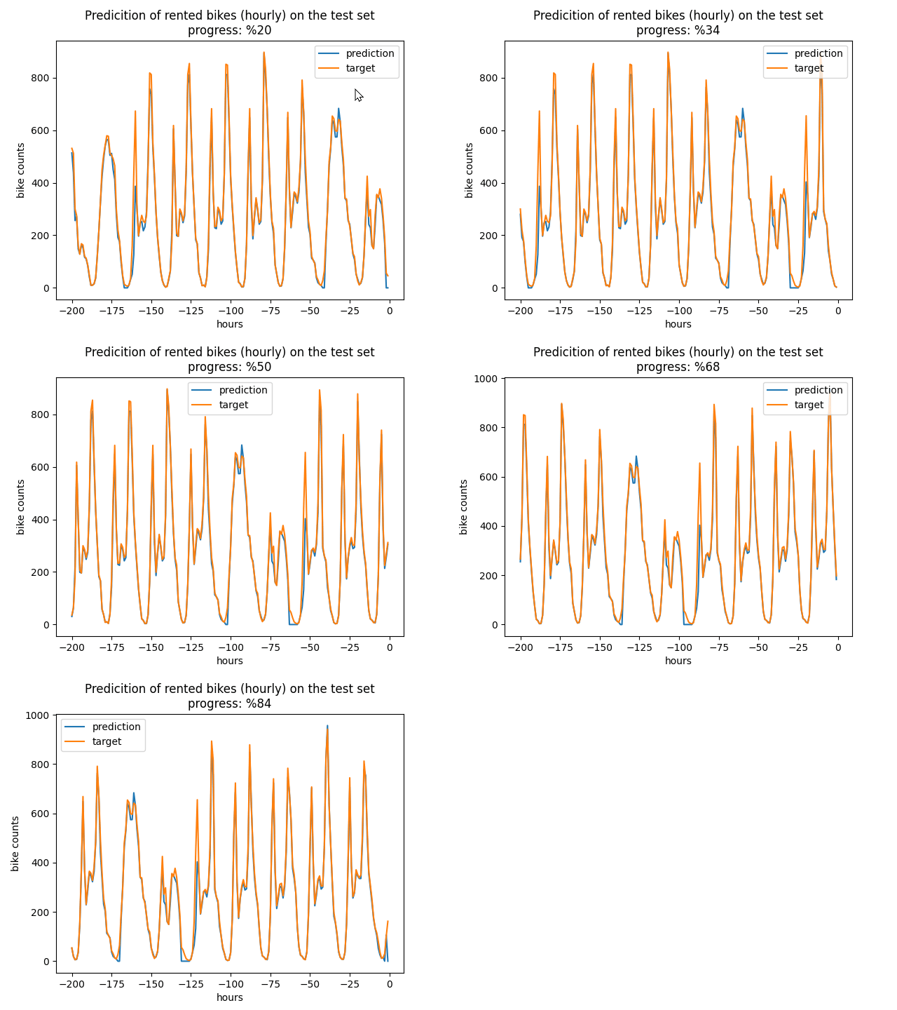
The predicted value and actual value for a portion of test set is shown in the figure below (with this configuration [[X(t-1), Y(t-25), Y(t-49)], [X(t), Y(t-24), Y(t-48)]]).

There are other hyperparameters which can be explored such as learning rate, batch size, num of bins, hidden size, number of layers, dropout, and reduced features. Also, different values can be tested for seqlen, day_num.